Climate Buffering of Marine Low Clouds
English Translation of Ebisuzaki 2023, TEN (Tsunami, Earth, and Networking), 4, 52-67 (in Japanese)
Toshikazu Ebisuzaki
Computational Astrophysics Laboratory, RIKEN (2-1, Horosawa, Wako, Saitama, 351-0198 Japan) E-mail: ebisu@riken.jp
Abstract
The buffering due to the cloud albedo effect of marine low clouds strongly stabilize the climate of the Earth. Marine low clouds cover the surface boundary layers (stratocumulus topped boundary layers: STBL) above the ocean with low surface temperature in the regions off the west coast of the continents. Low clouds strongly contribute to the cooling of the Earth due to their high albedo and large emissivity in the infrared wavelengths. The worming due to the increase in the concentration of the greenhouse gas starts at the troposphere-stratosphere boundary, and propagates down toward the sea surface. This downwardly propagating warming not only strengthens the temperature inversion, which prevents low cloud from their dissipation, but also creates new STBLs. The cloud coverage, as a result, significantly increases and cancels most of the temperature increase due to the greenhouse gas. This response of the atmosphere takes place in the timescale of radiative-convective equilibrium, which is hours to one day. When we consider this buffer effect of low clouds, the actual temperature increase in the surface of the ocean is found to be reduced to, at least, one third compared with the value without that effect. In other words, Earth’s average temperature increase is not 2.93 K for the case of doubling of CO2 concentration as Manabe and his colleagues argued but 0.98 K or less. Earth’s climate is strongly stabilized by this buffer effect of the ocean. The runaway in the climate will not take place, despite the warry of some researchers, as far as a significant fraction of the Earth is covered by the ocean.
Keywords
Climate change, Marine low cloud, Cloud albedo effect, Radiative-Convective equilibrium, Cloud topped boundary layer, Temperature Inversion layer, Aerosol, Global climate model
1. Introduction
The cloud albedo effect of marine low-level clouds buffers a large portion of temperature changes caused by the increase or decrease of greenhouse gases, strongly stabilizing the Earth’s climate. The cloud albedo effect is caused by a portion of the Earth’s surface being covered by clouds with high albedo. In particular, extensive and long-lasting marine low-level clouds off the west coasts of continents are a significant factor in increasing or decreasing the Earth’s albedo.
The present paper discusses climate change mitigation through the cloud albedo effect of low-level clouds. Here, clouds at a pressure of 700 hPa or more (below approximately 3 km in altitude) are referred to as low-level clouds, those at 400 hPa or less (above approximately 7 km in altitude) as high-level clouds, and those in between as mid-level clouds (Rossow and Shiffer 1990). Since the majority of low-level clouds are over the ocean, this paper focuses exclusively on marine low-level clouds.
Low-level clouds are entirely different from mid- and high-level clouds, as explained below (e.g., Kawai and Shige 2020). First, mid- and high-level clouds appear in locations with high sea surface temperatures (SSTs) and are often accompanied by precipitation. They are also associated with deep convective cells or warm fronts of extratropical cyclones, where the condensation of water vapor due to updrafts plays a crucial role. High-level clouds are often short-lived and do not significantly affect the Earth’s radiation budget.
In contrast, low-level clouds (stratus and stratocumulus) appear in areas with low sea surface temperatures (Klein and Hartmann 1993). They are rarely accompanied by strong winds or rain; at most, only light drizzle occurs. Since a temperature inversion layer forms in the lower troposphere, preventing dry downdrafts of the upper atmosphere from reaching near the sea surface. Meanwhile, the lower atmosphere below the inversion layer is trapped within the boundary layer, and water vapor from the sea surface becomes supersaturated, due to radiative cooling, leading to cloud formation. In the regions where low-level clouds are likely to appear (subtropical and some tropical areas off the west coasts of continents), the sea surface temperature is kept lower than in other regions at the same latitude due to the cold currents flowing in from the north and the coastal upwelling caused by Ekman transport.
The presence of low-level clouds has a strong cooling effect on the Earth. This is because they have high albedo, scattering most of the incoming solar visible light back into space, and they are strongly cooled by infrared radiation emitted from their warm cloud tops. The coverage fraction of marine low-level clouds is a critical factor in determining the global mean temperature (Klein and Hartmann 1993). Indeed, observations have shown that a slight change in the coverage fraction of marine low-level clouds can cause significant changes in the Earth’s climate (Wood 2012). For instance, a mere 3.5% to 5% increase in the global average area covered by low-level clouds has an effect that counteracts the effect caused by a doubling of carbon dioxide concentration (Randall et al. 1984; Slingo 1990). Since low-level clouds cover 40% of the Earth’s surface (Warren et al. 1986), this corresponds to a relative increase in low-level cloud cover of 8% to 12% (Wood et al. 2012)
In the present paper, we demonstrate that as the temperature in the upper atmosphere rises due to an increase in greenhouse gases, the coverage fraction of marine low-level clouds increases. The resulting cloud albedo effect then buffers a significant portion of the temperature increase caused by the rising greenhouse gas concentrations. This is revealed by assuming vertical radiative-convective equilibrium and using the empirical correlation between lower tropospheric stability (LSS) and cloud cover fraction. This buffering mechanism of the marine low-level cloud albedo effect is ignored in many studies evaluating the Earth’s heat budget, leading to an overestimation of the temperature increase caused by greenhouse gases. When this novel buffering mechanism is considered, the surface temperature increase is less than one-third of conventional estimates. This means that the Earth’s climate is strongly stabilized by the buffering effect of the ocean. The ‘runaway warming’ that many scholars worry about—where increasing CO2 concentrations reduce clouds and further accelerate warming—need not be a concern as long as the significant area of Earth is covered by oceans.
Section 2 explains the properties of marine low-level clouds as revealed by satellite observations, in situ measurements, and ground-based remote sensing, and uses these findings to clarify the mechanism by which warming in the upper atmosphere due to greenhouse gases increases low-level cloud cover fraction. In Section 3, we re-evaluate the increase in surface temperature caused by the increase in greenhouse gases, considering this climate change buffering. Section 4 discusses how variations in the Earth’s average temperature are determined by the interplay between stabilization from the cloud albedo effect and the snow-ice albedo effect, as well as the relationship with aerosol number density.
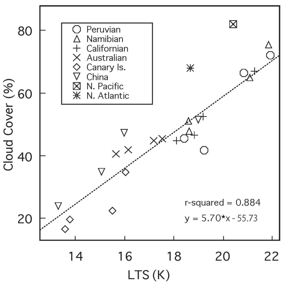
Figure 1. According to Klein and Hartman (1993), low cloud cover is strongly correlated with lower tropospheric stability (LTS) over many ocean regions on Earth (indicated by marks in the figure), based on a modification of Klein and Hartman (1993).
2. Properties of Marine Low-Level Clouds
2.1. Distribution Over the Ocean
Low-level cloud cover fraction is primarily determined by Lower Tropospheric Stability (LTS). Klein and Hartmann (1993) studied the global distribution of low-level clouds, including stratus, stratocumulus, and sky-obscuring fog, and revealed that these clouds extend off the west coasts of continents, such as off California, Peru, Namibia, and Mauritania. They also found a strong correlation between the low-level cloud cover fraction and the lower tropospheric stability, which is the difference in potential temperature between the 700 hPa pressure level and the sea surface (Figure 1). Potential temperature is the temperature a parcel of air would have if it were compressed adiabatically to a pressure of one atmosphere, and it is an indicator of atmospheric stability for convection. In particular, the atmosphere is stable when the potential temperature increases with height, and unstable when it decreases with height.
The oceans off the west coasts of continents have relatively low sea surface temperatures due to the cold currents from high latitudes and the coastal upwelling. On the other hand, the air temperature at the 700 hPa level maintains a uniform temperature in the longitudinal direction determined by latitude, leading to greater lower tropospheric stability in these regions.
Typical vertical profiles of temperature, cloud water content, and potential temperature in such regions are shown in Figure 2. A moist boundary layer just above the sea surface contains water vapor evaporated from the sea surface forms in the area close to the surface. Above this, a temperature inversion layer forms between this boundary layer and the air descending from the mid-to-upper atmosphere (above 700 hPa). Although the atmosphere typically cools with increasing altitude, the temperature increases within the inversion layer. The temperature difference (strength of the inversion layer) becomes larger as the sea surface temperature is lower or the lower tropospheric stability (LTS) is greater.
Across this inversion layer, dry, hot, and light (high-entropy) air that has descended from the mid-to-upper layers (above 700 hPa) exists in the upper zone, while moist, cold, and heavy (low-entropy) air is present in the lower zone. Because the atmospheric stratification is strongly stable against convection, air mixing across this layer is unlikely to occur. A boundary layer topped by such a stratocumulus cloud and temperature inversion layer is called a Stratocumulus-Topped Boundary Layer (STBL) (Wood 2012).
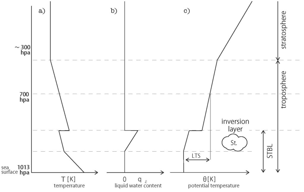
Figure 2. Typical vertical distribution of temperature (a), cloud water content (b), and potential temperature (c) in low sea surface temperature regions where low-level clouds are likely to form.
2.2. Mechanisms of Formation and Dissipation of marine low-level clouds
Marine low-level clouds are formed and maintained through the following processes (Duynkerke and Teixeria 2001; Wood 2012). Due to the strong temperature inversion layer immediately above the cloud-topped boundary layer, water vapor rising from the sea surface cannot mix into the dry downdrafts above the inversion layer. Consequently, the water vapor is trapped within the cloud-topped boundary layer, and water condenses due to nocturnal cooling, creating optically thick clouds in both visible light and infrared radiation. Strong cooling due to infrared radiation is concentrated within a few meters near the cloud top, which strengthens the temperature difference of the inversion layer (Figure 2a). Furthermore, the cold, heavy air masses created by this cooling sink, and in their place, air masses rise from the sea surface, leading to thorough mixing only within the cloud-topped boundary layer (the layer below the inversion layer). Air masses containing abundant water vapor from near the sea surface reach the dew point as they rise, and water condenses to form clouds. The release of latent heat further drives this ascent. The cloud water content increases proportionally to the height from the cloud base (Figure 2b). In this way, low-level clouds are maintained for a long time. During this ascent process, cloud particles gradually grow through water condensation, reaching their maximum size at the cloud top (Rosenfeld et al. 2019).
On the other hand, marine low-level clouds dissipate through the following two mechanisms. First, if the turbulence in the cloud-topped boundary layer is strong relative to the temperature difference of the inversion layer, an air parcel penetrates the temperature inversion layer, and dry air parcels from above intrude into the cloud layer. This phenomenon is called ‘entrainment’ of the upper atmosphere. When the dry, warm air parcel from the upper layer mixes with the cold, saturated air parcel in the cloud layer, latent heat is removed through the evaporation of cloud droplets, causing cooling. The parcel then becomes heavier than its surroundings, sinks further, and intrudes into the cloud-topped boundary layer. The cloud dissipates when such Cloud Top Entrainment Instability (CTEI) occurs (Deardroff 1980; Randall 1980; Kuo and Schubert 1988; Betts and Boers 1990; MacVean and Mason 1990; MacVean 1993; Yamaguchi and Randall 2008; Lock 2009; Noda et al. 2013).
Furthermore, as a result of the penetration of turbulent updrafts, the cloud top height increases. Consequently, the cloud water content at the cloud top becomes higher, and the cloud particle size increases. When this exceeds 14 μm, precipitation begins (Rosenfeld et al. 2019). When significant precipitation occurs, strong downdrafts are generated, dragged down by the falling cloud particles. This breaks the temperature inversion layer, promotes mixing (entrainment) with the upper layer, and triggers the aforementioned Cloud Top Entrainment Instability, leading to cloud dissipation (Wood 2012).
Conversely, when the lower tropospheric stability is high, neither of the two aforementioned cloud dissipation mechanisms functions, and marine low-level clouds are maintained over the long term. Figure 3 conceptually illustrates that as one moves westward from the west coast of a continent, the cloud morphology transitions and the physical processes governing them change. The right end of the figure corresponds to the coast off the west coast of a continent (off California in the North Pacific), where the lower tropospheric stability is high, while the left end corresponds to the central ocean (around Hawaii in the North Pacific), where the lower tropospheric stability is low. Within the subtropical oceanic high-pressure systems, downdrafts prevail. Near the west coasts of continents where the sea surface temperature is relatively low and the lower tropospheric stability is high (right end of Figure 3), low-level clouds develop through the mechanisms already described, completely filling the sky over the ocean without gaps. Naturally, the cloud cover fraction becomes very high.
However, in regions with high sea surface temperatures and low lower tropospheric stability (left end of Figure 3), the dissipation mechanisms mentioned above become effective, shortening the lifespan of low-level clouds and reducing their coverage fraction. Thus, as one moves westward, the cloud morphology sequentially changes from stratus to stratocumulus, closed convective cells, open convective cells, and scattered cumulus clouds as the sea surface temperature increases and the lower tropospheric stability decreases. Corresponding to these changes, the low-level cloud cover fraction decreases.
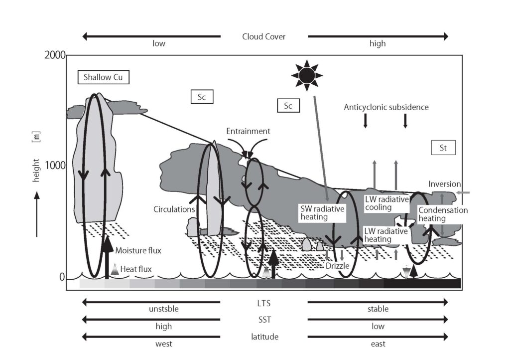
Figure 3. When the Lower Tropospheric Stability (LTS) is high, optically thick stratus clouds are formed (right end). As the LTS decreases, the cloud tops become higher, sequentially changing into stratocumulus (middle) and cumulus clouds (left end), and the cloud cover fraction decreases (modified based on Kawai and Shige 2020).
2.3. Summary
The development and dissipation of low-level clouds are determined by a complex interplay of factors: turbulence driven within the cloud-topped boundary layer by infrared cooling at the cloud top, visible light heating by the sun, water vapor supply from the sea surface, condensation in updrafts, and the difficulty of mass mixing through the temperature inversion layer. However, the nature that higher (lower) lower tropospheric stability or strength of the temperature inversion layer leads to the long-term survival (short-term dissipation) of high-albedo low-level clouds, thereby shifting the Earth’s heat budget towards cooling (heating), remains constant. In the next section, we will explain temperature buffering by the cloud albedo effect based on this principle.
3. Temperature Buffering by the Cloud Albedo Effect
In this section, we evaluate where the Earth’s heat budget settles when the air temperature increases due to factors such as an increase in greenhouse gas concentrations, considering the change in the coverage fraction of low-level clouds.
3.1. Earth’s Average Temperature
First, we explain the principles that determine the Earth’s average temperature. When a sphere of radius \(R\) made of a black body with no atmosphere is irradiated by visible light with a solar constant of F_0=1.37×10^3 [Wm-2], the heat balance equation is as follows:
\[
\pi R^{2} F_{0} = 4 \pi R^{2} \sigma T^{4} \tag{1}
\]
Here, \(\sigma = 5.67 \times 10^{-8}\ \mathrm{W\,m^{-2}\,K^{-4}} \) is the Stefan–Boltzmann constant, \(F_{0} = 1.37 \times 10^{2}\ \mathrm{W\,m^{-2}} \) is the solar constant, and \(T\) is the surface temperature of the sphere. Solving Equation (1) for \(T\) yields
\begin{equation}
T = \left( \frac{F_{0}}{4\sigma} \right)^{1/4}
= T_{0} = 2.79 \times 10^{2}\ \mathrm{K}.
\tag{2}
\end{equation}
The \( T \) obtained in this way represents the average temperature of the Earth’s surface. Now, while the Earth can be approximated as a black body for infrared radiation, it is not a black body for visible light. That is, it does not absorb all the incident visible light, but reflects a certain proportion back into space. Since an atmospheric layer exists near the Earth’s surface, and some of the infrared radiation emitted from the surface is absorbed and retained there, the temperature of the atmospheric layer near the surface is higher than the temperature calculated using Equation \( (2) \) (the greenhouse effect). Considering these effects, the Earth’s surface temperature \( T \) can be calculated as follows:
\[
T=T_0[(1+\tau_*)(1-A)]^{1/4} \tag{3}
\]
Here, \( A \) is the Earth’s albedo, representing the fraction of incident visible light that is not absorbed but returned to space. For the actual Earth, it is said to be between \( 0.3 \) and \( 0.4 \). The albedo depends on factors such as the fraction of continents, cloud cover, and ice sheet cover.
On the other hand, \( \tau_* \) is a parameter representing the strength of the greenhouse effect. When the atmospheric optical thickness \( \tau \) for infrared radiation is much smaller than \( 1 \), \( \tau_* \) approximately matches \( \tau \). Conversely, when \( \tau \) is larger than about \( 1 \), the atmosphere becomes unstable for convection, and heat from the surface is transported by convection rather than infrared radiation. In this regime, \( \tau_* \) is an increasing function of \( \tau \) but has a smaller value than \( \tau \).
Since the atmospheric \( \tau \) strongly depends on the amount of water vapor it contains, it varies greatly by location and time. The global average is around \( 5\text{–}7 \), and the effective \( \tau_* \) is about \( 0.5 \). Substituting \( A = 0.35 \) and \( \tau_* = 0.5 \) into Equation \( (3) \) yields \( T = 270\ \mathrm{K} \). Linearizing Equation \( (3) \):
\[
\Delta T=T_0\frac{(1-A)\Delta \tau_*-(1+\tau_*)\Delta A}{4} \tag{4}
\]
Here, \( \Delta \tau_* \) and \( \Delta A \) are the deviations from the standard values. The hypothetical temperature increase \( \Delta T_{\mathrm{GH}} \) caused only by the change in greenhouse gas concentration (assuming no change in albedo) is:
\[
\Delta T_{\mathrm{GH}} = T_{0} \, \frac{(1 – A)\,\Delta \tau_*}{4} \tag{5}
\]
Here, \( \Delta T_{\mathrm{GH}} \) can be calculated as follows. Manabe and Wetherald (1975), under conditions neglecting ocean heat transport and fixing cloud conditions, solved the radiative-convective equilibrium at each global point and coupled it with atmospheric flow to determine the equilibrium temperature for both standard (\( 300\ \mathrm{ppm} \)) and doubled (\( 600\ \mathrm{ppm} \)) carbon dioxide concentrations. They obtained a global average temperature difference of \( 2.93 \) degrees between the two cases, which corresponds to \( \Delta T_{\mathrm{GH}} \) in Equation \( (5) \). This means
\[
\Delta T_{\mathrm{GH}} = 2.93\ \mathrm{K} \tag{6}
\].
Here, we assume that \( A \) is a function of temperature, and its partial derivative with respect to temperature is denoted as \( \partial A / \partial T \). Therefore,
\[
\Delta A = \frac{\partial A}{\partial T}\,\Delta T \tag{7}\]
Substituting this into Equation \( (4) \) and solving for \( \Delta T \), the solution, denoted as \( \Delta T_{\mathrm{RCE}} \), represents the temperature change after radiative–convective equilibrium is established:
\[
\Delta T_{\mathrm{RCE}} = \frac{\Delta T_{\mathrm{GH}}}{1 + T_{0}\,\frac{(1+\tau_*)}{4}\,\frac{\partial A}{\partial T}} \tag{8}
\]
(Slingo et al. 1990).
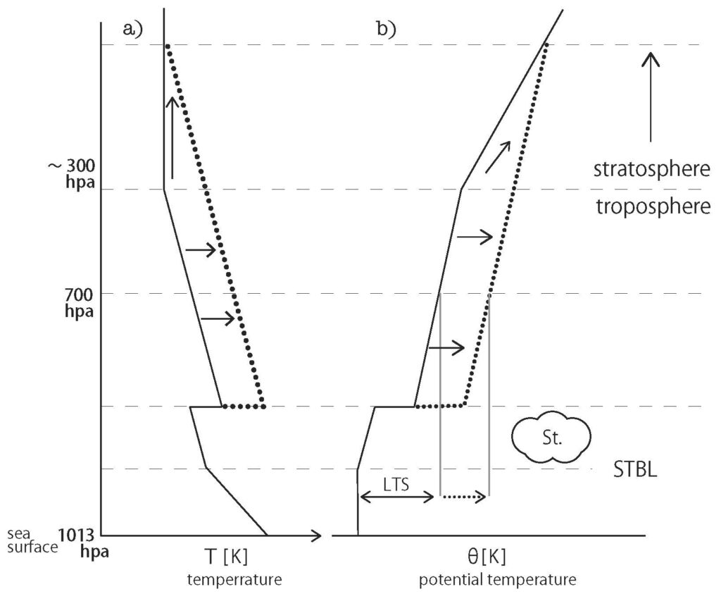
Figure 4. An increase in greenhouse gases leads to changes in potential temperature and air temperature, causing the tropopause to rise. This results in increased air and potential temperature above the cloud-topped boundary layer, occurring on a short timescale (a few hours) as the atmosphere reaches radiative-convective equilibrium. Sea surface temperature with its high thermal inertia, however, does not respond, so that the temperature difference in the temperature inversion layer. This process enhances lower tropospheric stability (LTS), which is the potential temperature difference between the 700 hPa level and the sea surface, ultimately allowing low-level clouds like stratus and stratocumulus to persist longer.
3.2. Temperature Change Resulting from Increased Greenhouse Gas Concentrations
In this section, we conduct a thought experiment on how the atmosphere reacts when the atmospheric greenhouse gas concentration increases simultaneously and instantaneously everywhere. The Earth’s atmosphere has a structure with the stratosphere overlying the troposphere. In the latter, the atmosphere is opaque to infrared radiation and most heat is transported by convection, while in the former, it is transparent to infrared radiation and most heat is transported by radiation. At an altitude of about 10 km is the stratosphere, the boundary between the two layers. Thus, the stratosphere-troposphere boundary cab be defined as where the dominant mode of heat transport changes from convection to radiation, or where the atmosphere changes from opaque to transparent to infrared radiation. Physically, these two definitions are nearly equivalent. Near the stratosphere-troposphere boundary, the temperature is in radiative equilibrium with the infrared radiation balancing the heat input from the sun, so the temperature barely changes as long as the solar heat input does not change. On the other hand, the increase in greenhouse gas concentration has little effect, since most heat is transported by convection in the troposphere. However, the position of the boundary between the two layers shifts upward (towards lower pressure) in response to the increase in the infrared absorption coefficient. This change occurs in a very short time scale from the moment of the change in greenhouse gas concentration (the time it takes for light to cross the thickness of the atmosphere, about 100 microseconds). This corresponds to the radiative equilibrium timescale. At this point, the warming occurs only near the stratosphere.
In this manner, when the temperature at a given pressure level increases (warming) near the stratosphere-troposphere boundary, the atmospheric stability for convection increases, convection weakens, and heat transport by convection stagnates, causing the temperature in the layer below to rise. This warming region then propagates down into the lower troposphere. If this warming wave reached the ground or the sea surface, it would result in warming at the ground or sea surface. This change corresponds to convective equilibrium, and all of these changes occur on the timescale of an air parcel circulating through the troposphere (the time it takes for an air parcel moving at several meters per second to cross the thickness of the atmosphere: generally, about one hour).
Let’s discuss the impact of this warming on the Earth’s surface (sea surface) at the bottom of the atmosphere, divided into two cases: when a temperature inversion layer (cloud-topped boundary layer) is present in the lower troposphere, and when it is not. First, consider the case where a temperature inversion layer originally exists. As discussed by Wood (2017), in regions where the sea surface temperature is low relative to the atmosphere (off the west coasts of continents: off California, Chile, Mozambique, etc.), a temperature inversion layer forms in the lower troposphere (P<700 hPa), and below it exists a ‘cloud-topped boundary layer’ (CTBL) that is strongly coupled thermally with the sea surface and covered at the top by stratus clouds. Cooling at this upper surface of the clouds maintains the turbulence within the cloud-topped boundary layer and the temperature inversion layer itself. Since the temperature inversion layer is strongly stable against convection, the propagation of warming from the upper atmosphere via convection stops here, and the cloud-topped boundary layer below is isolated from the warming. As a result, the temperature difference of the inversion layer increases, making it even more stable against convection (Figure 4). The transport of heat and substance through the temperature inversion layer occurs via the entrainment caused by the penetration of turbulent updrafts, but this is further suppressed by the strengthening of the inversion layer, leading to an increase in cloud cover fraction as the stratus clouds cover the sea surface for a long time (Subsection 2.2).
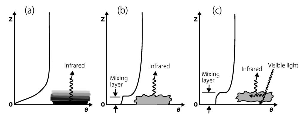
Figure 5. Fog formation in the surface layer. (a) As the temperature of the surface layer downs by the infrared cooling, it reaches to the dew point to form clouds (fogs). Fog layer is most dense at the surface and become thinner as altitude increase. The upper layer is not clear. (b) Cooling become large at the cloudtop (radiative cooling instability) to create a new stratocumulus topped boundary layer. Cool dense air subdrafts to mix with the air of lower layers, which makes cloud layers uniform. As a result, the top boundary become clear. (c) If the CTBL become optically thick enough to infrared and optical radiation during nighttime, it can survive daytime even if it is exposed to the heating from the Sun(modified based on Stull 1988)。
On the other hand, in the regions where the sea surface temperature is high relative to the atmosphere (such as the eastern half of oceans), strong convection is excited by the input of heat and water from the ocean surface heated by daytime solar radiation. The temperature inversion layer is broken, and the entire tropospheric layer is well mixed. Convection is usually intermittent (mostly in the afternoon), and for most of the period, the sky is clear without clouds, and the atmosphere is nearly neutral regarding convection. In such regions, the warming reaches the upper part of the surface layer, a few tens of meters above the sea surface. Turbulence is excited in the surface layer due to the wind over the ocean. This turbulence transports heat downward and water vapor upward.
When the temperature of the upper surface of the surface layer rises due to warming, the atmosphere stabilizes against the vertical movement of air parcels, turbulence is suppressed, and the thermal coupling with the atmosphere above via turbulence weakens. As a result, as the warm water layer on the sea surface disappears due to nocturnal infrared cooling, the temperature of the surface layer drops, reaching the dew point, and clouds (fog) form (Figure 5a). Their thickness is often very thin, only 1 to 5 meters. The density of the fog is also non-uniform; it is densest just above the sea surface, becomes thinner with increasing height, and its upper boundary is indistinct (Stull 1988; Figure 5a). Since liquid water has a higher radiative efficiency for infrared radiation compared to water vapor, further cooling proceeds (radiative cooling instability). As a result of cold air parcels sinking and mixing due to cooling, the fog layer becomes uniform, and its upper boundary becomes distinct (Figure 5b). A cloud-topped boundary layer that has developed sufficiently both upward and downward during the night becomes optically thick to visible light as well. At this point, it can be maintained for a long time without dissipating even when exposed to daytime solar heating. As the air temperature rises, the cloud base lifts off the ground (Figure 5c), forming a new cloud-topped boundary layer. The formation of such new cloud-topped boundary layers increases the cloud cover fraction.
This mechanism of low-level cloud formation is similar to the phenomenon of ‘cold sea fog’ (e.g., Koracin et al. 2014), which occurs when warm, moist air flows over cold water. In the case of cold sea fog, warm air flows in from the horizontal direction, but in the case of increasing greenhouse gas concentrations, the warming comes from above. Cold sea fog was formalized in studies of the ‘Hot Spell’ event off the west coast of North America, where hot air flows from land to sea causing dense fog (Pilie et al. 1979), and is considered the most common mechanism of sea fog formation (Koracin et al. 2014). Similar phenomena are observed in the ‘Harr’ event on the east coast of Scotland (Taylor 1987) and sea fog in the Yellow Sea (Zhang et al. 2009).
To summarize the mechanisms described above, the warming of the atmosphere from above due to an increase in greenhouse gas concentrations strengthens the temperature inversion layer where it already existed, and newly creates a temperature inversion layer in areas where it did not exist before. As a result, cloud cover fraction increases in all regions. This increase in low-level clouds occurs on the timescale of reaching convective equilibrium (generally a few hours). Even including the formation of new cloud-topped boundary layers due to nocturnal cooling, it concludes within 24 hours. Therefore, the Earth’s albedo increases due to the warming caused by increased greenhouse gases. That is, ∂A/∂T in Equation 8 is positive, and its absolute value is quite large. In other words, the Earth’s atmosphere has a very strong negative feedback (i.e., a buffering effect) against temperature changes caused by rising carbon dioxide concentrations (Figure 6a).
On the other hand, Miller (1997) conducted a thought experiment very similar to this section. He divided the ocean into three regions: regions with high (warm) sea surface temperatures and developing convection, those without, and regions with relatively low (cold) sea temperatures. Assuming equilibrium of heat and water budgets in these three regions, he calculated the change in sea surface temperature when carbon dioxide concentration doubled and obtained a result where the sea surface temperature of the cold ocean slightly increased. Based on this result, the lower tropospheric stability, marine low-level cloud cover fraction, and the Earth’s albedo all decrease, which means a positive feedback (amplification effect) occurs with increasing sea surface temperature (Figure 6b). Therefore, it was concluded that there is a risk of the Earth’s surface temperature becoming unstable, leading to runaway warming.
However, a problem with this calculation lies in the use of a coarse vertical grid spacing of 100m when solving the radiative-convective equilibrium in each region to determine the changes in the distribution of vertical physical quantities (temperature, cloud water content, etc.). As explained in detail in Subsection 3.3, the increase in stratus cloud cover fraction due to the increased temperature difference in the inversion layer is ignored unless careful calculations are performed using a dense vertical grid spacing of a few meters.
Furthermore, the equilibrium of heat and water budgets from the warm ocean to the cold ocean assumed in this paper is not realistic. Considering that the warm and cold oceans are thousands of kilometers apart and it takes several days just for an air parcel to travel that distance, and that due to the very large thermal inertia of seawater, it takes at least a week (depending on the flow conditions below the sea surface) for the sea surface temperature to change significantly due to heat conduction from the atmosphere, such an equilibrium state would take at least several weeks to establish. The vertical radiative-convective equilibrium in the atmospheric layer (Figure 4 and Figure 6a) is established much faster than that. Without considering this, the ‘Miller (1997) equilibrium state’ will never occur in the real atmosphere. Similar problems also exist in past assessments by Manabe and his followers (e.g., Manabe et al. 1990; Stouffer and Manabe 1999). The correct method for evaluating the impact of phenomena occurring on such long time-scales on climate change will be discussed in Subsection 4.2
Hartmann and Klein (1993), based on observational data, derived the correlation formula between low-level cloud cover \( C_f \) and lower tropospheric stability
\( \theta_1 – \theta_0 \):
\[
C_f = 5.70(\theta_1 – \theta_0) – 55.73
\tag{9}
\]
Here, we obtain a change in low-level cloud cover of \( \partial C_f / \partial T = 0.057\ \mathrm{K^{-1}} \) corresponding to a one-degree change in lower tropospheric stability (Figure 1). Here, \( \theta_1 \) is the potential temperature at \( 700\ \mathrm{hPa} \) pressure,
and \( \theta_0 \) is the potential temperature at sea level. From the discussion in Subsection 2.2, \( \Delta \theta_1 = \Delta T \) and \( \Delta \theta_0 = 0 \). Furthermore, if \( \eta \) is the ratio of the sea area where the low-level cloud cover \( C_f \) is determined by the lower tropospheric stability to the total ocean area:
\begin{eqnarray}
\frac{\partial A}{\partial T}
&=& 0.71\,\eta \,[A_{\mathrm{cloud}} – A_{\mathrm{sea}}]\,
\frac{\partial C_f}{\partial T}\\
&\sim& 2.0 \times 10^{-2}
\left( \frac{\eta}{0.7} \right)
\left( \frac{A_{\mathrm{cloud}} – A_{\mathrm{sea}}}{0.7} \right)
\ \mathrm{K^{-1}}
\tag{10}
\end{eqnarray}
We obtain the following. \( A_{\mathrm{cloud}} \) and \( A_{\mathrm{sea}} \) are the cloud and sea surface albedos, respectively. Using the value of the ocean area as \( 71\% \) of the total Earth surface area, and typical values of \( 0.8 \) (Seinfeld and Pandis1997) and
\( 0.1 \) (Jin et al. 2011; Kalish and Mackle 2012; Huang et al. 2019) for \( A_{\mathrm{cloud}} \) and \( A_{\mathrm{sea}} \), respectively, we get the following. Substituting Equation \( (10) \), \( T_0 = 279\ \mathrm{K} \), and \( \Delta \tau_* = 0.5 \) into Equation \( (8) \), we obtain:
\[
\Delta T_{\mathrm{RCE}}
= \frac{\Delta T_{\mathrm{GH}}}
{1 + 2.1
\left( \frac{\eta}{0.7} \right)
\left( \frac{A_{\mathrm{cloud}} – A_{\mathrm{sea}}}{0.7} \right)}
\tag{11}
\]
Assuming \( \Delta T_{\mathrm{GH}} = 2.93\ \mathrm{K} \) (Equation \( (6) \)), we obtain \( \Delta T_{\mathrm{RCE}} = 0.98\ \mathrm{K} \). This means that the temperature increase for a doubling of CO\(_2\) concentration is not \( 2.93\ \mathrm{K} \), but rather \( 0.98\ \mathrm{K} \), approximately one-third of the value after reaching radiative–convective equilibrium, considering the negative feedback due to the albedo effect of low-level clouds. This ratio is rather conservative, since (1) the temperature increase propagating from the upper layer should actually follow the dry adiabatic lapse rate instead of the wet adiabatic lapse rate assumed here, and (2) only the increase in the cover fraction of existing cloud-topped boundary layers is considered here, not the formation of new cloud-topped boundary layers, which will be discussed in detail in Subsection 3.3. It is highly likely that \( \Delta T_{\mathrm{RCE}} \) will become even smaller.
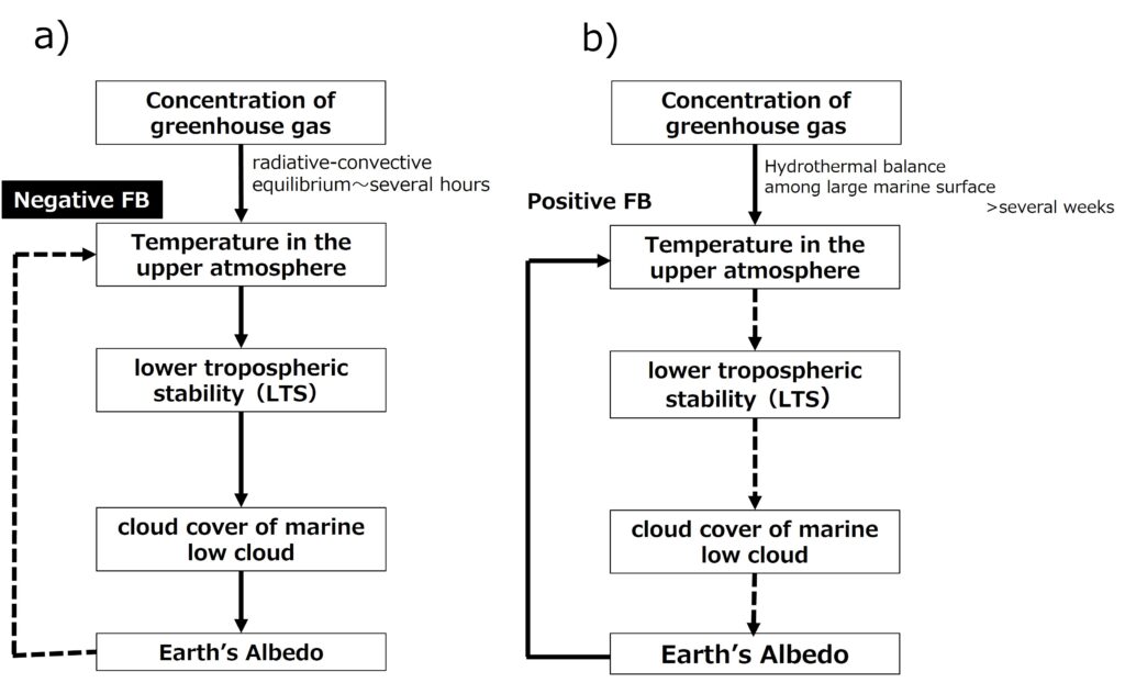
Figure 6. Two different perspectives on the response of the Earth’s atmospheric layer to the increase in greenhouse gas concentrations. Solid arrows represent positive feedback, and dashed arrows represent negative feedback. a) In this paper, we assume that vertical radiative-convective equilibrium in the atmosphere is established first when greenhouse gas concentration increases. As a result, the temperature of the mid-to-upper atmosphere, lower tropospheric stability, marine low-level cloud cover fraction, and Earth’s albedo all increase, leading to a negative feedback on the mid-to-upper atmospheric temperature. Radiative-convective equilibrium is reached in at least a few hours, which is overwhelmingly faster than the rate at which heat and water balance through the atmosphere across the widespread ocean surface is established. Therefore, the temperature increase due to increased greenhouse gas concentrations is buffered and stabilized by the increase in marine low-level clouds. In contrast, b) Miller (1995) assumed that when greenhouse gas concentration increases, the temperature of cold oceans would rise when the heat and water budget equilibrium through the atmosphere over the wide ocean surface. As a result, the lower tropospheric stability, marine low-level cloud cover fraction, and Earth’s albedo all would decrease, which would result in a positive feedback on the sea surface temperature. Consequently, it was concluded that there wpuld be a risk of the Earth’s surface temperature becoming unstable, leading to runaway warming. Unfortunately, because he ignored the important changes in low-level clouds explained above (a), his conclusion is incorrect.
3.3. Why Can Global Climate Models Not Reproduce the Distribution of Marine Low-Level Clouds?
The basic properties of marine low-level clouds described in Subsection 2.2 have been clarified and already established through the development of global observations using satellites, in situ measurements using aircraft, and ground-based remote sensing. Therefore, if a simulation were executed using a numerical calculation code that correctly represents these properties, the climate buffering due to variations in marine low-level cloud cover fraction as described in this paper should be observed.
However, the inability of global climate models to adequately represent the distribution of marine low-level clouds off the west coasts of continents has long been a problem (Duynkerke and Teixeria 2001; Siebesma et al. 2004). Even current climate models cannot successfully reproduce observations of subtropical stratocumulus clouds off the west coasts of continents (Nam et al. 2012; Caldwell et al. 2013; Su et al. 2013; Koshiro et al. 2018). Lauer and Hamilton (2013) reported that the simulation results of CMIP3 and CMIP5 underestimate the cloud cover fraction in subtropical stratocumulus regions and have a large bias in the shortwave radiation effect. In fact, they overestimate the sea surface temperature off the west coasts of continents by as much as 5 K, partly because they fail to represent the marine stratocumulus clouds in these regions properly (Ma et al. 1996; Duynkerke and Teixeria 2001).
Marine low-level clouds are also important for local, short-term phenomena. For example, the ‘Yamase’ phenomenon that occurs in Japan is accompanied by the Yamase wind from the northeast and marine stratocumulus clouds (Kodama 1997; Kodama et al. 2009; Koseki et al. 2012; Shimada et al. 2014). When the Okhotsk High Pressure system appears in the summer, northeasterly winds prevail along the Pacific coast of the Tohoku region of Japan. At this time, stratocumulus clouds form off the coast of Tohoku and are transported to the Pacific coast of the Tohoku region. The air temperature in this region drops dramatically due to the cold north wind and the blocking of solar radiation. Until a few hundred years ago, crop yields plummeted due to this low temperature, and many people starved to death. It is known that the stratocumulus clouds accompanying this Yamase phenomenon cannot be reproduced by numerical weather forecasts.
This problem stems from the coarse vertical resolution (vertical grid spacing) of global climate models, which is typically 100-300m. To correctly reproduce the cloud-topped boundary layer in numerical calculations, it is necessary to resolve both the temperature inversion layer at the top (including the cloud-top cooling layer) and the surface layer at the bottom using a fine vertical grid spacing of a few meters. The cooling layer at the cloud top is only a few meters thick. Although this layer is considered to have an average width of several tens of meters in the horizontal direction, this is due to the irregularities at the cloud top, and the thickness of the cooling layer at any given location is only a few meters.
If one attempts to represent this with a coarse grid spacing of 100 m or more, the magnitude of the infrared cooling, which should occur intensely within a few meters, is averaged out to about 1/100th of its actual value. This leads to an underestimation of the generation rate of cold, heavy air masses and results in weak, intermittent turbulence characteristic of the cloud-topped boundary layer. Furthermore, because the temperature gradient in the inversion layer is underestimated by nearly a factor of 100, the penetration of turbulent updrafts and the resulting top-down entrainment are overestimated, creating a strong bias towards the rapid dissipation of stratus clouds.”
Furthermore, the surface layer, which is only a few tens of meters thick and is the location where the cloud-topped boundary layer is generated, also cannot be represented accurately. If it is represented with a coarse grid spacing of 100 meters or more, the formation of fog, which should originally start at the very bottom of the surface layer due to nocturnal cooling, cannot be represented with sufficient accuracy. The onset of this fog and the accompanying turbulence, which should occur at a height of about 10 m above the ground (sea surface), are strongly suppressed. This is because the forced averaging due to the coarse grid spacing makes it impossible to represent the eigenmode with the maximum growth rate of the radiative cooling instability that generates new cloud-topped boundary layers.
In fact, Koracin et al. (2005) attempted to reproduce dense fog caused by a hot spell event (Subsection 3.2) using one-dimensional numerical simulations. They used grid points of 180 points (average spacing of approx. 6.7 m), 90 points (average spacing of approx. 13 m), and 45 points (average spacing of approx. 27 m) between the ground and 1200 m altitude. In the simulations that used only 90 or 45 points, the distribution of cloud water content—that is, the occurrence of fog—did not match the relatively high-precision calculation using 180 points, not even qualitatively, let alone quantitatively. This indicates that at least a vertical grid spacing of a few meters is necessary for the reproduction of cold sea fog due to radiative cooling instability. It is considered that the same applies to reproducing the formation of fog (new cloud-topped boundary layers) caused by the warming of the upper atmosphere associated with the increase in greenhouse gas concentrations.
A strange bias exists in global climate models where errors in the radiation budget cancel each other out—for instance, by generating fewer low-level clouds and more high-level clouds (Nam et al. 2012). This is because the parameters in global climate models are tuned so that the heat budget is generally balanced over decades and warming occurs with only a slight amount of heating (Mauritsen et al. 2012; Hourdin et al. 2013; Hourdin et al. 2017). Nam et al. (2012) also pointed out that even when looking solely at low-level clouds, a bias of “Too few, too bright” exists (underestimating cloud cover while overestimating cloud albedo). This situation has not improved even recently (Konsta et al. 2022).
To clarify the reality of the strange biases found in such global climate models, particularly the behavior of low-level clouds, Hein and Hentgen (2021) investigated the behavior of subtropical marine low-level clouds in a high-resolution simulation (where horizontal grid spacing was refined to a few kilometers to allegedly resolve convective cells). To increase the horizontal resolution, the simulation was limited to the region off the coast of Mozambique in the Atlantic Ocean, where marine low-level clouds are likely to spread due to low sea surface temperatures. As a result, the cloud patterns generated changed systematically both qualitatively and quantitatively as the horizontal resolution increased, but this change stopped when the resolution became finer than 2.2 km. This indicates that the typical size of deep convective cell systems is about 10 km, and their basic properties can be reproduced with sufficient accuracy if the grid spacing is about one-fifth of that size. This property, where the simulation accuracy improves as the grid spacing is reduced and physical quantities converge to a certain value without showing abnormal fluctuations, is called ‘convergence’ in numerical computation science. This convergence is considered a fundamental issue that should be confirmed first to perform ‘meaningful’ simulations with high predictability. In the case of climate models, the simulation cannot be trusted unless the horizontal grid spacing is at least around 2.5 km.
However, even in high-resolution calculations using regional or local weather models with small horizontal grid spacing as described above, the reproducibility of low-level clouds varies greatly depending on the model and the size of the grid spacing (e.g., Kawai and Shige 2020). This means that a 2.5 km horizontal grid spacing is insufficient to converge the calculation results for reproducing low-level clouds. Hein and Hentgen (2021) did not examine convergence by varying the vertical grid, but stated that they used vertical grid spacing of 20 m at the surface layer (0 km altitude) and 180 m at 1 km altitude. This is several times (surface layer) to tens of times (1 km altitude) coarser than the grid spacing required by the physical processes of low-level cloud formation and dissipation explained above. This grid spacing is dense enough for simulating deep convective cells but insufficient for handling the cloud-topped boundary layer, which has layers where physical quantities change rapidly in the vertical direction (the temperature inversion layer and the surface layer). Naturally, the important values do not converge under these conditions. Furthermore, in global climate simulations, which have coarser grid spacing in both horizontal and vertical directions than regional or local weather models, it is impossible to know what is actually happening.
It is unfortunate that studies investigating the reaction of the Earth’s atmosphere when greenhouse gas concentrations suddenly increase are being eagerly conducted using such coarse-grid global climate models (e.g., Gregoly et al. 2004; Zelinka et al. 2013; Qu et al. 2014; Qu et al. 2015; Bretherton 2015; Bretherton and Blossey 2014; Zelinka et al. 2019). Their results vary widely, ranging from those where clouds decrease and warming proceeds runaway, to those where clouds decrease and warming is suppressed in response to the increase in carbon dioxide concentration (e.g., Kawai and Shige 2020).
This is a natural consequence considering that all these studies use models whose computational convergence (as described above) has not been confirmed. We have already explained that even global climate models claiming ‘ultra-high resolution’ (e.g., Bretherton 2015; Bretherton and Blossey 2014) have still insufficient in vertical grid spacing. Despite the fact that there is only one true answer, they are analyzing the distribution of various global climate simulation results and trying to obtain something resembling an answer by taking an average. They should bear in mind that no matter how much they analyze calculation results full of errors, they can only understand numerical errors (which naturally may include systematic biases that do not disappear through averaging).
The only solution to this confused situation is to continue the effort to obtain the one and only true answer by performing true high-resolution global climate simulations that adopt sufficiently fine grid spacing in both the horizontal and vertical directions. If this will be done, the atmospheric response where low-level clouds increase in response to the increase in greenhouse gas concentrations, as described in Figure 5a, should be stably observed, and at the same time, the convergence of the calculation results should be confirmed.
4. Discussion
In this paper, we clarified the properties of marine low-level clouds, which have a large impact on the Earth’s heat budget, in Section 2, and explained that their coverage fraction strongly correlates with lower tropospheric stability (LTS). LTS is the difference in potential temperature between the 700 hPa pressure level (approximately 3 km altitude) and the sea surface. When LTS is high, the temperature difference of the temperature inversion layer formed at the boundary of the cloud-topped boundary layer increases, trapping moisture from the sea surface within the cloud-topped boundary layer and filling its top with low-level clouds over a long period.
In Section 3, considering these properties of low-level clouds, we clarified that an increase in greenhouse gas concentration leads to a rise in the temperature of the mid-to-upper atmosphere, rather than the sea surface temperature. This strengthens LTS and increases the coverage fraction of marine low-level clouds.
In this section, we discuss the Earth’s temperature variations based on these findings.
4.1. Variations in Earth’s Average Temperature
The Earth’s average temperature is strongly stabilized by the cloud albedo effect resulting from the increase or decrease of marine low-level clouds. This is consistent with our daily observations of temperature changes. The temperature in a certain location is constantly fluctuating, but a few weeks of high temperatures are typically followed by a few weeks of low temperatures, and the range of variation decreases as longer averages are taken. When averaged over a year, the range of variation becomes very small. This is a typical characteristic of a stable system with negative feedback. In contrast, in a system with positive feedback, the variations would be much more intense, and the range of variation would hardly decrease even with long-term averaging.
In reality, in addition to the cloud albedo effect discussed here, there is also the snow-ice albedo effect. This effect stems from the fact that a portion of the Earth’s surface is covered by snow and ice (which have high albedo). When the surface temperature is low (high), the area covered by snow and ice increases (decreases), which increases (decreases) the Earth’s albedo, leading to further increases (decreases) in snow and ice coverage. Thus, the snow-ice albedo effect provides positive feedback to the Earth system and contributes to the instability of the Earth’s temperature. Indeed, it is known that during cold periods when the Earth’s average temperature is low and large areas are covered by snow and ice (typically ice ages), the variations in the Earth’s average temperature are large (e.g., Gradstein et al. 2020).
In summary, it can be said that the Earth’s temperature is stabilized by the cloud albedo effect over low-latitude oceans and destabilized by the snow-ice albedo effect at high latitudes. The larger temperature changes observed at high latitudes can be seen as a manifestation of this.
We also clarified in Section 3 that the increase in greenhouse gas concentrations produces a secondary effect that increases low-level clouds, and the actual temperature increase is limited to about one-third or less compared to the case where the cloud albedo effect is not considered. Most of the ‘global warming’ caused by greenhouse gases is counteracted by this buffering effect of the ocean. In response to a doubling of carbon dioxide concentration, the Earth’s average temperature will not rise by 2.93 K as claimed by Manabe and Wetherald (1975), but will remain below 0.98 K. The Earth’s average temperature is strongly stabilized by this powerful buffering effect of the ocean. Therefore, the runaway warming that many scholars worry about (e.g., Steffen et al. 2020) need not be a major concern as long as the Earth has oceans.
4.2. Aerosol Number Density
Low-level cloud cover is also sensitive to the aerosol number density in the air (e.g., Rosenfeld et al. 2006). When the number density of aerosol particles is high, the cloud particles that form around them as nuclei are smaller in size and greater in number. This has two effects. First, for the same liquid water path, the optical thickness for visible light increases and the albedo rises, which weakens daytime visible light heating (Twomey 1977). Second, because the particles are smaller and their cross-sectional area and relative velocity with the air are lower, it takes longer to reach the minimum effective radius (about 14 µm) required for precipitation to occur. As a result of these two effects, a higher aerosol number density causes low-level clouds to be maintained for a longer time, and the cloud cover fraction becomes higher.
Rosenfeld et al. (2019) therefore conducted a more careful data analysis of oceanic meteorological data between the equator and 40 degrees south latitude, performing a cautious separation of the effects that lower tropospheric stability (LTS), cloud geometric thickness, and cloud particle density have on the low-level cloud cover fraction. The result revealed that the low-level cloud cover fraction strongly depends not only on LTS but also on the aerosol number density, represented by the cloud particle density. In this case, Equation 8 becomes:
\[
\Delta T_{\mathrm{RCE}}
=
\frac{
\Delta T_* –
T_{0}\,\frac{(1+\tau_*)}{4}\,
\frac{\partial A}{\partial N}\,\Delta N
}{
1 +
T_{0}\,\frac{(1+\tau_*)}{4}\,
\frac{\partial A}{\partial T}
}
\tag{12}
\]
An increase in aerosol number density can increase the coverage fraction of marine low-level clouds and lead to global climate cooling. For example, Turco et al. (1983) warned that the increase in aerosols caused by a nuclear war could lead to a global cooling (nuclear winter). However, it should be noted that due to the buffering effect of marine low-level clouds discussed in Section 3, the impact of this cooling is reduced to about one-third, similar to the case of temperature increase caused by greenhouse gases.
The origins of aerosols over the ocean can be considered as: (1)those from sea salt particles generated by wave breaking, (2)those from dust transported from continents, (3) those of anthropogenic origin from ships and industrial areas, and (4)those from sulfate aerosols produced by the photo-oxidation of organic sulfides (mainly dimethylsulfonic acid) released by marine plankton. Charlson et al. (1987) (the CLAW paper) argued that the aerosol number density in the open oceanis dominated by those originating from organic sulfides from marine plankton, and they considered that their proliferation is positively dependent on temperature, such that\( \Delta N_{\mathrm{CLAW}} = (\partial N / \partial T)_{\mathrm{CLAW}} \, \Delta T > 0 \).
If this feedback (which we call the CLAW effect here) is realized on a short timescale similar to radiative–convective equilibrium (a few hours),
Equation \( (12) \) becomes:
\[
T_{\mathrm{RCE}}
=
\frac{
\Delta T_* –
T_{0}\,\frac{(1+\tau_*)}{4}\,
\frac{\partial A}{\partial N}\,
\Delta N_{\mathrm{nonCLAW}}
}{
1 +
T_{0}\,\frac{(1+\tau_*)}{4}\,
\left[
\frac{\partial A}{\partial T}
+
\frac{\partial A}{\partial N}
\left( \frac{\partial N}{\partial T} \right)_{\mathrm{CLAW}}
\right]
}
\tag{13}
\]
In other words, as discussed by Lovelock (1979), the CLAW effect contributes to the buffering of the Earth’s climate. However, as discussed in Section 2.2, it is thought that the sea surface temperature where the phytoplankton inhabit does not change significantly on a timescale of a few hours, so the CLAW effect might not be that large. In fact, Ayers and Cainey (2007) state that although many studies have been conducted since the proposal of the CLAW hypothesis, it is difficult to say that it has been quantitatively verified.
If the feedback due to the CLAW effect occurs on a longer timescale of several days or more, the two factors are separated, so Equation \( (13) \) becomes:
\begin{eqnarray}
T_{\mathrm{RCE}}
&=&
\frac{
\Delta T_* –
T_{0}\,\frac{(1+\tau_*)}{4}\,
\frac{\partial A}{\partial N}\,
\Delta N_{\mathrm{nonCLAW}}
}{
1 +
T_{0}\,\frac{(1+\tau_*)}{4}\,
\frac{\partial A}{\partial T}
}\\
&\times&\left(
1 +
T_{0}\,\frac{(1+\tau_*)}{4}\,
\frac{\partial A}{\partial N}
\left( \frac{\partial N}{\partial T} \right)_{\mathrm{CLAW}}
\right)
\tag{14}
\end{eqnarray}
Other factors than the CLAW effect—such as the “Miller 1997 equilibrium” discussed in Section 3.2—were to be established, those effects should be considered as a factor multiplying the first factor representing the buffering effect due to radiative–convective equilibrium, like the second factor in the denominator on the right-hand side of Equation \( (14) \).
The discussion on the aerosol number density over the ocean is not straightforward, since it is determined by a complex interplay of human activities, cosmic ray flux, marine biological production, and the climate itself, including precipitation. As there is insufficient space to unravel and explain these causal links here, we will discuss this in a separate paper.
Acknowledgments
We would like to express our gratitude to Dr. Yasushi Take, Dr. Taishi Sugiyama, and Dr. Genki Katada for their valuable comments and suggestions during the writing of this paper. The initial draft of the English translation was produced using GPT-5.2.
Reference
1) Ayes, C.P. and J.M. Cainey, 2007, The CLAW hypothesis: a review of the major developments, Environ. Chem., 4, 366-374.
2) Betts, A.K., and R. Boers, 1990, A cloudiness transition in a marine boundary layer. J. Atmos. Sci., 47, 1480–1497.
3) Caldwell, P.M., Y. Zhang, and S. A. Klein, 2013, CMIP3 subtropical stratocumulus cloud feedback interpreted through a mixed-layer model. J. Climate, 26, 1607–1625.
4) Charson, R.J., J.E. Lovelock, M.O. Andreae, and S.G. Warren, (CLAW), 1987, Oceanic phytoplankton, atmospheric sulphur, cloud albedo and climate, Nature, 326, 665-661.
5) Deardorff, J. W., 1980, Cloud top entrainment instability. J. Atmos. Sci., 37, 131–147.
6) Duynkerke, P. G., and J. Teixeira, 2001: Comparison of the ECMWF reanalysis with FIRE I observations, Diurnal variation of marine stratocumulus. J. Climate, 14, 1466‒1478.
7) Gregory, J.M. et al., 2004, A new method for diagnosing radiative forcing and climate sensitivity, Geophyisical Research Letters, 31, L03205.
8) Gradstein, F.M. et al., 2020, Geologic Time Scale 2020 volume 2, Elsevier.
9) Guev, S.G., 1997, Climatologically significant effects of space-time averaging in the north Atlantic sea-air heat flux fields, Journal of Climate, 10, 2743-2763.
10) Heim、C. and Hentgen, L. 2021, Inter-model Variability in Convection-Resolving Simulations of Subtropical Marine Low Clouds, Journal of the Metological Society of Japan, 99, 1271-1295.
11) 11) Hourdin F. et al. 2013, LMDZ5B: the atmospheric component of the IPSL climate model with revisited parameterizations for clouds and convection, Clim. Dyn, 40, 2193-2222.
12) Hourdin F. et al. 2017, The art and science of climate model, Bulletin of the American Metheologcal Society, 3, 589-603.
13) Huang, C.J. et al. 2018, Observation and Parameterization of broadband sea surface albedo, Journal of Geophysical Research-Oceans, 124, 4480-4491.
14) Jin, Z.H. et al., 2011, A new parameterization of spectral and broadband ocean surface albedo, Optics Express 19, 26429-26443.
15) Kalisch, J and Macke, A, 2012, Radiative budget and cloud radiative effect over the Atlantic from ship-based observations, Atmospheric Measurement Techniques, 5, 2391-2401.
16) Kawai, H. and Shige, S., 2020, Marine low cloud and their parameterization in climate models, Journal of the Meteorological Society of Japan, 98, 1097-1127.
17) Klein, S. A., and D. L. Hartmann, 1993, The seasonal cycle of low stratiform clouds. J. Climate, 6, 1587‒1606.
18) Kodama, Y., 1997: Airmass transformation of the Yamase air-flow in the summer of 1993. J. Meteor. Soc. Japan, 75, 737–751.
19) Kodama, Y.-M., Y. Tomiya, and S. Asano, 2009: Air mass transformation along trajectories of airflow and its relation to vertical structures of the maritime atmosphere and clouds in Yamase events. J. Meteor. Soc. Japan, 87, 665–685.
20) Koseki, S., T. Nakamura, H. Mitsudera, and Y. Wang, 2012, Modeling low-level clouds over the Okhotsk Sea in summer: Cloud formation and its effects on the Okhotsk high. J. Geophys. Res., 117, D05208.
21) Komori, S. et al., 2018, Laboratory measurements of heat transfer and drag coefficients at extremely high wind speeds, Journal of Physical Oceanology, 48, 959-974.
22) Konsta D. et al., 2021, Low-level Marine tropical clouds in six CMIP6 models are too few, too bright but also too compact and too homogeneous, Geophysical Research Letters, 49, 11, 10.1029/2021GL097593.
23) Koracin et al. 2005, Modeling sea fog on the U.S. California coast during a hot spell event, Geofizika, 22, 59-81.
24) Koracin, D. et al. 2014, Marine fog: A review, Atmospheric Research, 143, 142-175.
25) Koshiro, T., M. Shiotani, H. Kawai, and S. Yukimoto, 2018, Evaluation of relationships between subtropical marine low stratiform cloudiness and estimated inversion strength in CMIP5 models using the satellite simulator package COSP. SOLA, 14, 25–32.
26) Kuo, H.-C., and W. H. Schubert, 1988, Stability of cloud topped boundary layers. Quart. J. Roy. Meteor. Soc., 114, 887–916.
27) Lauer, A., and K. Hamilton, 2013: Simulating clouds with global climate models: A comparison of CMIP5 results with CMIP3 and satellite data. J. Climate, 26, 3823–1123 3845.
28) Lock, A. P., 2009, Factors influencing cloud area at the capping inversion for shallow cumulus clouds. Quart. J. Roy. Meteor. Soc., 135, 941–952.
29) Lovelock, J. 1979, GAIA, a new look at life on Earth, Oxford University Press.
30) Ma, C.-C., C. R. Mechoso, A. W. Robertson, and A. Arakawa, 1996: Peruvian stratus clouds and the tropical Pacific circulation: A coupled ocean-atmosphere GCM study. J. Climate, 9, 1635–1645.
31) MacVean, M. K., 1993, A numerical investigation of the criterion for cloud-top entrainment instability. J. Atmos. Sci., 50, 2481–2495.
32) MacVean, M. K., and P. J. Mason, 1990, Cloud-top entrainment instability through small-scale mixing and its parameterization in numerical models. J. Atmos. Sci., 47, 1012–1030.
33) Manabe, S., Bryan, K., Spelman, J. 1990, Transient response of a global ocean-Atmospheric model to a doubling of atmospheric carbon dioxide, Journal of Physical Oceanology, 20, 722-749.
34) Manabe, S. and Weatheraid, 1997, Thermal equilibrium of the atmosphere with given distribution of relative humidity, Journal of the Atmospheric Sciences, 24, 241-259.
35) Miller, R. L., 1997, Tropical thermostat and low cloud cover, Journal of Climate, 10, 409-440.
36) Mauritsen T. et al. 2012, Tuning the climate of a global model, J. Adv. Model. Earth Syst., 4, M00A01.
37) Nam, C., S. Bony, J.-L. Dufresne, and H. Chepfer, 2012, The too few, too bright tropical low-cloud problem in CMIP5 models. Geophys. Res. Lett., 39, L21801.
38) Noda, A. T., K. Nakamura, T. Iwasaki, and M. Satoh, 2014, Responses of subtropical marine stratocumulus cloud to perturbed lower atmospheres. SOLA, 10, 34–38.
39) Pilie R.J. et al., 1979, The formation of marine for and the development of fog-strutus systems along the California coast, Journal of Applied Meteorology, 18, 1275-1286.
40) Randall, D. A., 1980, Conditional instability of the first kind upside-down. J. Atmos. Sci., 37, 125–130.
41) Randall, D. A., 1984, Stratocumulus cloud deepening through entrainment. Tellus, 36A, 446–457.
42) Rosenfeld, D., Y. J. Kaufman, I. Koren, 2006, Switching cloud cover and dynamical regimes from open to closed Benard cells in response to the suppression of precipitation by aerosols, Atmos. Chem. Phys. 6, 2503–2511.
43) Rosenfeld, D., Zhu, Y., Wang, M., Zheng, Y., Goren, T., Yu, S., 2019, Aerosol-driven droplet concentrations dominate coverage and water of oceanic low-level clouds, Science, 363, 599.
44) Rossow, W. B., and R. A. Schiffer, 1999, Advances in understanding clouds from ISCCP, Bull. Amer. Meteor, Soc., 80, 2261‒2287.
45) Seinfeld, J. H., and S. N. Pandis, 1997: Atmospheric Chemistry and Physics: From Air Pollution to Climate Change. Wiley-Interscience, p994.
46) Steffen, W., Richardson, K., Rockstrom, J., Joachim, H., Dube, O.P., Dutreuil, S., Lenton, T.M., Lubchenco, J., 2020, The emergence and evolution of Earth system science, Nature Reviews, Earth and Enviroment, 1, 54-63.
47) Stouffer, R.J., Manabe, S., 1999, Response of a ocean-atmospheric model to increasing atmospheric carbon dioxide: sensitivity to the rate increase, Journal of Climate, 12, 2224-2237.
48) Shimada, T., M. Sawada, and T. Iwasaki, 2014, Indices of cool summer climate in northern Japan: Yamase indices, J. Meteor. Soc. Japan, 92, 17–35.
49) Siebesma, A. P., C. Jakob, G. Lenderink, R. A. J. Neggers, J. Teixera, E. Van Meijgaard, J. Calvo, A. Chlond, H. Grenier, C. Jones, M. Köhler, H. Kitagawa, P. Marquet, A. P. Lock, F. Müller, D. Olmeda, and C. Serverijns, 2004: Cloud representation in generalcirculation models over the northern Pacific Ocean: A EUROCS intercomparison study. Quart. J. Roy. Meteor. Soc., 130, 3245‒3267.
50) Slingo, A., 1990: Sensitivity of the Earth’s radiation budget to changes is low clouds. Nature, 343, 49–51.
51) Su, H., J. H. Jiang, C. Zhai, V. S. Perun, J. T. Shen, A. D. Del Genio, L. S. Nazarenko, L. J. Donner, L. W. Horowitz, C. J. Seman, C. J. Morcrette, J. Petch, M. A. Ringer, J. Cole, M. d. S. Mesquita, T. Iversen, J. E. Kristjansson, A. Gettelman, L. D. Rotstayn, S. J. Jeffrey, J.-L. Dufresne, M. Watanabe, H. Kawai, T. Koshiro, T. Wu, E. M. Volodin, T. L’Ecuyer, J. Teixeira, and G. L. Stephens, 2013: Diagnosis of regimedependent cloud simulation errors in CMIP5 models using “A-Train” satellite observations and reanalysis data. J. Geophys. Res.: Atmos., 118, 2762–2780.
52) R.B. Stull, An Introduction to Boundary Layer Meteorology, 1988, Kluwer Academic Press.
53) Taylor W., 1987, Mesoscale case study: Project haar, Met Office Met. O.111 Tech note 239.
54) Twomey, S., 1977, The influence of pollution on the shortwave albedo of clouds, J. Atmos. Sci., 34, 1149-1152.
55) Turco, R.P.; Toon, O.B.; Ackerman, T.P.; Pollack, J.B.; Sagan, C. 1983, Nuclear Winter: Global Consequences of Multiple Nuclear Explosions, Science 222, 4630
56) Warren, S. G., C. J. Hahn, J. London, R. M. Chervin, and R. L. Jenne, 1986: Global distribution of total cloud cover and cloud types over land. NCAR Tech. Note NCAR/TN-2731STR, National Center for Atmospheric Research, Boulder, CO, 29 pp. 1 200 maps.
57) Wood, R., 2012, Stratocumulus clouds. Mon. Wea. Rev., 140, 2373–2423.
58) Yamaguchi, T., and D. A. Randall, 2008, Large-eddy simulation of evaporatively driven entrainment in cloud topped mixed layers. J. Atmos. Sci., 65, 1481–1504.
59) Zelinka M.D. et al. 2013, Contributions of different cloud types to feedbacks and rapidadjustment in CMIP5, J. Climate, 26, 5007-5027
60) Zhang S. et al., 2009, Seasonal variation of Yellow Sea fog: observation and mechanism, J. Clim., 22m 6578-6772.
 |
TEN vol.4
|

科学はひとつ 宇宙物理学者による知的挑戦の記録
戎崎俊一 著
学而図書/四六判 並製320頁/本体2,400円+税
12年にわたり「戎崎の科学は一つ」で執筆されてきた記事を精選し、「地震と津波防災」など全9章に再編。すべての章に著者書き下ろしの解説を加えて集成した一冊。